Natural Language Processing (NLP) Models are able to receive an input of text and convert each individual word or token into a number which can then be modeled and analyzed in terms of linear distance and relationship to other tokens. There are many different architectures and parameters which go into the creation of an NLP model and can have substantial impact on model accuracy as well as model training time. When testing many different model configurations optimizers such as nAdam, Adam, and RMSprop can increase accuracy and minimize training time, lowering the risk of failure. Encoders, which convert words into tokens, and embedding layers also can also have an impact on the model’s ability to understand the words fed into the network. Regularization can assist in the training of models which have high dimensionality in the training set, “controlling” the weight sizes and the management of the error. LSTM and RNN layers can give a model “memory” to allow it to learn the context of an input—an important step in NLP since context is important both within a sentence and within the text from which the training data is derived. Convolutional layers as well as dense layers also impact model training convergence, accuracy, and fit (or overfitting). Finally, the algorithm to choose the number of nodes in each of these layers is important and can impact the ability of the model to learn complex relationships between features; due to the complexity and nuance of language different methods of choosing these values, such as though the use of the Fibonacci sequence, doubling, halving, or setting the values to be equal, are all options worth considering. Ultimately however the decision of model architecture comes down to the tradeoff between training time to convergence and accuracy, or the time/computational cost of a model, and a parsimonious model is preferable to a complex model based on the value of performance.
Language has been described as the “jewel in the crown of cognition” (Pinker, 1994) and while there are many ways in which entities in nature communicate, humans are the only known life-form to possess “language.” (University of Minnesota, 2010) As such it should be no surprised that language is also highly complex and nuanced, often contained multiple “levels of meaning”, making its modeling by traditional methods difficult. Linguistic statements are comprised of compounding series of elements and in many languages, particularly English, series order is important. In this paper I shall examine several kinds of methods used to model language, or natural language processing (NLP), using neural networks, specifically models which incorporate single and deep fully connected layers, convolutional layers, recurrent layers such as long short-term memory (LSTM) and bi-directional LSTM layers. I shall also experiment with different regularizers, the use of the Fibonacci sequence in model construction, and encoding structures which convert words in a lexicon to numbers and works with an embedding layer which maps those numbers to a lookup table in a multi-dimensional space.
Language itself, and with-it cognition, has arguably been at the center of philosophical inquiry since the beginning of Western philosophy, and is central subject of many philosophical treatises. For many linguists, language is not simply a communication device by which humans signal intent or meaning; the “Sapir-Whorf Hypothesis” is a combination of two theories presented separately by E. Sapir and B. L. Whorf which (contentiously) posits that language is not simply referential, but acts as both an architecture as well as a medium of experience for the human mind; “The central idea of the Sapir-Whorf hypothesis is that language functions, not simply as a device for reporting experience, but also, and more significantly, as a way of defining experience for its speakers.” (Hoijer, 1954) The ability for an artificially intelligent agent to be able to process and “understand” language is thus of paramount importance, and indeed even integral to some definitions of “Artificial Intelligence” (viz. the “Turing Test” presented by Alan Turing in the “Computing Machinery and Intelligence”). (Turing, 1950) In the Turing Test, an agent is found to be intelligent if their use of language is indistinguishable from that of a human actor. In other words, for Turing, the processing, understanding, and use of language is the cornerstone of human intelligence and indicative of “thought.” After the invention of the neural network, model architectures which take the complexity as well as the nuance of language into account is the second step toward achieving general machine intelligence.
Aside from the philosophical endeavor to not only understand human language but create an artificially intelligent agent which is capable of doing the same, NLP models offer great benefits to business, organizations, and government entities by gaining the ability to not only process large amounts of linguistic statements at scale, but make inferences from these statements using methods such as sentiment analysis and subject classification, perform subject summarization and data extraction, or even construct chat agents capable of assisting humans, allowing users to use the same natural language they would use to communicate with a human agent.
There are risks however to the implementation of NLP models, or more specifically implementing a poor NLP model. Studies show that humans have a negative bias against artificially intelligent agents and are more critical of their performance than they are of a human agent performing the same task (Vedantm, 2015); due to both the complexity of language, the central role that language plays in both communication as well as thought, and our disproportionate bias against error caused by artificially intelligent agents its imperative that machine learning architects spend time ensuring optimal NLP model performance.
Much has been written about the use of recurrent neural networks (RNN), convolutional neural networks (CNN), and long short-term memory (LSTM) models implemented in order to classify text and the performance evaluation of these models. J. Cai compared the difference between RNN and CNN in both time and precision and found that in some cases the CNN models outperform the RNN models both in terms of training time and precision. (Cai et al., 2018) Hybrid CNN and LSTM architectures were tested for news article classification with a LSTM CNN architectures with word embeddings obtaining higher accuracy than LSTM, Bidirectional LSTM, CNN, CNN/LSTM, and CNN/Bi-Directional-LSTM models alone. (Shi et al., 2019) Similarly, RNN and CNN modeling methods (CRAN) have been developed to compensate with relatively shallow CRANs outperforming very deep CNN models (Guo et al., 2018; Shi et al., 2019) and Bi-directional LSTM models can increase the F1 score relative to CNN, LSTM, and support vector machines (SVM) by providing additional context and introducing less noise. (Li et al., 2018) In their exploration of using Bidirectional LSTM models for tagging the number of tokens alone in Bidirectional LSTM models do not predict performance.(Wang et al., 2015) The efficacy of regularization and the application of dropout layers on embeddings, activations, and LSTM model weights, combined with averaged stochastic gradient descent (ASGD) where the returned values from SDG are averaged over K iterations showed significant improvement over manual tuning of an LSTM model, and regularization by weight-dropping showed significant gains over optimization. (Merity et al., 2017) In several experiment simple word-embedding models (SWEM) showed superior performance to CNN and RNN models, leading to the suggestion that max pooling and hierarchical pooling to word embeddings within models; (Shen et al., 2018)
The application of the Fibonacci sequence to neural networks, specifically to weight values, while using the golden ratio as a learning rate was found to improve the learning curve of the models.(Luwes, 2010) Fibonacci Neural Networks (FNN) have been built which implement the Fibonacci polynomial equation within the activation function itself and found it to be superior to solving fractional order advection reaction-diffusion equations (FRDE), a kind of partial differential equation which is used to model phenomena in statistical physics, neuroscience, and economics and for which an exact solution is often both desirable and elusive due to the complexity.(Dwivedi & Rajeev, 2021) The use of Fibonacci polynomial equations in classification using multi-layer perceptrons which traditionally have performance degradation for high dimensional data has been suggested in order to increase the accuracy, sensitivity, precision, and specificity of the network while reducing the computational complexity in applications concerning high dimensional medical data, specifically when compared to Naïve Bayes, Ada Boost, SVM, and Bayes net models.(Maqsood et al., 2021)
Three sets of experiments with 11 independent variables were performed and in total 160 Models were created, trained, and graded. First the dataset used for training was obtained and preliminary EDA was preformed to determine the total number of unique tokens and general distribution of the four categories. The data was then split into a training, validation, and test set which was consistent for each of the experiments., and the distribution of the training sets were examined to minimize classification bias. Each of the experiments were designed and infrastructure was developed to support the design, construction, compilation, training, evaluation, and analysis of each of the modes.
Many of the experiments explored the use of the Fibonacci sequence, ether directly or by mapping a set of numbers to the Fibonacci sequence. The Fibonacci sequence is a sequence of numbers where the next number in the sequence is equal to the sum of the previous two numbers as seen in equation 1. The series, along with the closely related golden ratio, is often found in nature and often used in applications to represent increasing magnitudes of complexity.
In several of the variables in this experiment a sequence of values were created which used projection of the Fibonacci sequence in order to create a set of n-numbers that matched the proportions of the Fibonacci set. To accomplish this I created several formulas, first to generate my sequence, and then to scale the variables to be used as model hyper-parameters.
					def get_fibonacci_sequence(x, n = 1, factor = 1, in_place = True, counting = False):
        def checkif_fibonacci(number):
            if number != 0:
                a = math.sqrt(5*number**2 + 4)
                b = math.sqrt(5*number**2 - 4)
                truth_value = (a % 1 == 0 or b % 1 == 0)
            elif number == 0:
                truth_value = True
            return (truth_value)

        def get_fibonacci_number(place):
            if place != 0:
                Phi = (1 + math.sqrt(5)) / 2
                phi = -1/Phi
                number = math.floor((Phi**place - phi**place) / math.sqrt(5))
            elif place == 0:
                number = 0
            else:
                raise ValueError("Must be zero or a positive integer.")
            return (number)

        def get_fibonacci_by_place(starting_place, length_of_sequence):
            container = []
            for i in range (starting_place, starting_place + length_of_sequence):
                container.append(get_fibonacci_number(i))
                i += 1
            return (container)

        fibonacci = []

        if in_place == True:
            # n indicates starting place in sequence
            fibonacci = get_fibonacci_by_place(n, x)

        else:
            # n indicates starting number
            if checkif_fibonacci(n) == False:
                raise ValueError(f"{n} is not a Fibonacci number. Set 'in_place' to true if n indicates starting position.'")

            else:
                fibonacci_set = []
                j = 0

                while n not in fibonacci_set:
                    fibonacci_set.append(get_fibonacci_number(j))
                    j += 1

                place = fibonacci_set.index(n)

                fibonacci = get_fibonacci_by_place(place, x)

        if counting == True and fibonacci.count(1) > 1:
            fibonacci.remove(1)
            if x > 2:
                fibonacci.append(fibonacci[-1] + fibonacci[-2])
            elif x == 2:
                fibonacci.append(2)

        return ([number * factor for number in fibonacci])
#Example
print("First 10 fibronacci counting numbers beginning with the 6th number:",get_fibonacci_sequence(10, n = 6, in_place = True, counting = True))
print("First 7 fibronacci numbers beginning with 0:",get_fibonacci_sequence(7, n = 0, in_place = False))
print("First 5 fibronacci numbers starting with 55:",get_fibonacci_sequence(5, n = 55, in_place = False))
First 10 fibronacci counting numbers beginning with the 6th number: [8, 13, 21, 34, 55, 89, 144, 233, 377, 610]
First 7 fibronacci numbers beginning with 0: [0, 1, 1, 2, 3, 5, 8]
First 5 fibronacci numbers starting with 55: [55, 89, 144, 233, 377]
					def scale_fibonacci(x, max_value, count = True):
        fibonacci_sequence = get_fibonacci_sequence(x = x, counting = True)
        unit = max_value/fibonacci_sequence[-1]
        scaled_sequence = []
        for number in fibonacci_sequence:
            scaled_sequence.append(math.ceil(unit * number))
        return (scaled_sequence)
The dataset selected for the experiments was provided by Keras TensorFlow and was a collection of news article headlines compiled by the ComeToMyHead academic news search engine. The dataset was split into three equally distributed training, test, and validations sets; the training set contained 120,000 observations, the validation set contained 6400 observations, and the test set contained 1200 observations. The headlines and the target class containing the proper subject matter of the headline (Business, Sports, World, or Sci/Tech) were combined into TensorFlow datasets.
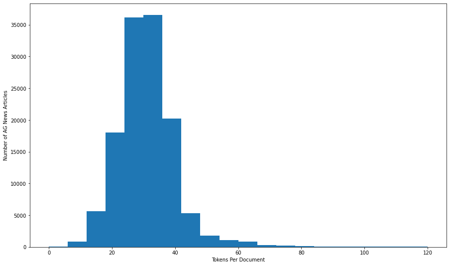
In total, the corpus of 127,600 news headlines contained 90,800 vocabulary words (tokens) and 3,909,695 words; each headline contained between 3 and 173 tokens.
A pipline was created to shuffle the order of the observations in the training set every epoch and create batch sizes of 64 tensors.
| description | label | |
|---|---|---|
| 0 | AMD #39;s new dual-core Opteron chip is designed mainly for corporate computing applications, including databases, Web services, and financial transactions. | 3 (Sci/Tech) |
| 1 | Reuters - Major League Baseball\Monday announced a decision on the appeal filed by Chicago Cubs\pitcher Kerry Wood regarding a suspension stemming from an\incident earlier this season. | 1 (Sports) |
| 2 | President Bush #39;s quot;revenue-neutral quot; tax reform needs losers to balance its winners, and people claiming the federal deduction for state and local taxes may be in administration planners #39; sights, news reports say. | 2 (Business) |
| 3 | Britain will run out of leading scientists unless science education is improved, says Professor Colin Pillinger. | 3 (Sci/Tech) |
| 4 | London, England (Sports Network) - England midfielder Steven Gerrard injured his groin late in Thursday #39;s training session, but is hopeful he will be ready for Saturday #39;s World Cup qualifier against Austria. | 1 (Sports) |
| 5 | TOKYO - Sony Corp. is banking on the $3 billion deal to acquire Hollywood studio Metro-Goldwyn-Mayer Inc... | 0 (World) |
| 6 | Giant pandas may well prefer bamboo to laptops, but wireless technology is helping researchers in China in their efforts to protect the engandered animals living in the remote Wolong Nature Reserve. | 3 (Sci/Tech) |
| 7 | VILNIUS, Lithuania - Lithuania #39;s main parties formed an alliance to try to keep a Russian-born tycoon and his populist promises out of the government in Sunday #39;s second round of parliamentary elections in this Baltic country. | 0 (World) |
| 8 | Witnesses in the trial of a US soldier charged with abusing prisoners at Abu Ghraib have told the court that the CIA sometimes directed abuse and orders were received from military command to toughen interrogations. | 0 (World) |
| 9 | Dan Olsen of Ponte Vedra Beach, Fla., shot a 7-under 65 Thursday to take a one-shot lead after two rounds of the PGA Tour qualifying tournament. | 1 (Sports) |
Experiment 1 was concerned with the size of the encoders and the impact on accuracy and training time. All of the encoders were trained on the original corpus with no modification to the data other than stripping all punctuation and replacing upper case letters with the lower case using TensorFlow’s TextVectorization object.
Four encoders were created using the Fibonacci scaling formula function. The encoders contained 18160, 36320, 54480, and 90800 words.
					def build_encoder(encoder_x, db, tokens):
        encoder_x = tf.keras.layers.experimental.preprocessing.TextVectorization(
            max_tokens = tokens,
            standardize = 'lower_and_strip_punctuation',
            output_mode = 'int',
            output_sequence_length = 64
        )
        encoder_x.adapt(db.map(lambda text, label: text))
        encoder_output = encoder_x
        vocab = np.array(encoder_output.get_vocabulary())
        vocab_length = len(vocab)
        return (encoder_output, vocab_length)
					i = 0
for encoder in encoder_set:
    encoder_set[encoder_names[i]], length = build_encoder(
        encoder_set[encoder],
        db = dataset_all,
        tokens = encoder_sequences[i]
        )

    print ("Encoder object:",encoder_set[encoder])
    print ("Encoder name:",encoder_names[i])
    print ("Vocab length:", length)
    print ()
    i = i + 1
Encoder object: <tensorflow.python.keras.layers.preprocessing.text_vectorization.TextVectorization object at 0x7fe25868a150>
Encoder name: encoder_18160
Vocab length: 18160

Encoder object: <tensorflow.python.keras.layers.preprocessing.text_vectorization.TextVectorization object at 0x7fe25838d490>
Encoder name: encoder_36320
Vocab length: 36320

Encoder object: <tensorflow.python.keras.layers.preprocessing.text_vectorization.TextVectorization object at 0x7fe27815c590>
Encoder name: encoder_54480
Vocab length: 54480

Encoder object: <tensorflow.python.keras.layers.preprocessing.text_vectorization.TextVectorization object at 0x7fe258b2d690>
Encoder name: encoder_90800
Vocab length: 90800
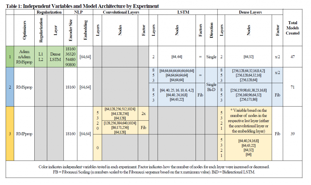
The first experiment was conducted testing the performance of the test set accuracy and the test set loss based on (a) different lengths of encoders (determined using a method I have called Fibonacci scaling where the number of words is determined based on the Fibonacci series, scaled such that a series of four values was generated, the fourth being equal to the total number of words, (b) the kind of regularize applied, and (c) the layer upon which the regularize was applied. Experiment 1 focused on the independent variables of optimizers, regularizers, layers being regularized, and the encoder size.
The second experiment primarily tested the LSTM layers, namely if (a) performance was impacted by bidirectional layers or single layers, (b) the number of LSTM layers present (using the Fibonacci sequence to determine test values), (c) the number of dense layers (using the Fibonacci sequence), and (d) if the reduction of the number of dense nodes was from layer to layer was based on halving or if the Fibonacci sequence was again used.
The third experiment was setup to primarily act as a “baseline” experiment to use convolutional networks or dense networks rather than LSTM or RNN models; the (a) number of convolutional layers, (b) number of dense layers, and (c) the increment of the convolutional layers was tested (either by doubling or by scaling using the Fibonacci sequence). Note that since there were models created without any convolutional layers this experiment also tested a pure dense neural network. Model configurations by experiment and variable can be found in Table 1.
Additional parameters which had been previously tested, such as the optimizer used in experiment 1, were kept consistent in experiment 2 and experiment 3, based on the results of the previous experiment. Each model’s performance was scored and the results were analyzed using (a) Pearson’s correlation, (b) the correlation between the correlations (again using Pearson’s method), (c) the coefficients of the variables predicting (a) test accuracy, (b) test loss, and (c) model training time, and confusion matrices subset by (a) encoder, (b) regularizer, and (c) layer.
Pairwise models for each possible combination of variables had to be created, which resulted in a total of 160 models being trained. In order to construct, train, and test such a high number of models the ‘model sets’ were created programatically using functions to construct, compile, backup, train, test, and analyze the models. Backup procedures were built into the model training functions so that the performance metrics of training models could be restored from backup.
Variable dictionaries containing each of the configuration parameters for the independent variables were created and then used to program the hyperparameters for each model, the size of the encoder (experiment 1), architecture, optimizer used, and unique name. Often, as in the example below, the variable dictionary’s value was calculated programmatically (in this case using the Fibonacci generator).
					experiment_3_ind_var = {
    'Encoder' : 'encoder_18160',
    'LSTM_direction' : ['None'],
    'LSTM_n' : ['None'],
    'LSTM_layers' : [0],
    'Convolution_layers' : get_fibonacci_sequence(5,
        n = 0,
        factor = 1,
        in_place = False,
        counting = True
        )[::-1],
    'Convolution_increase' : ['Doubled','Fibonacci'],
    'Dense_layers' : get_fibonacci_sequence(4,
        n = 1,
        factor = 1,
        in_place = False,
        counting = True)[::-1],
    'Reduction_factor' : ["Fibonacci"]
}
experiment_3_ind_var
{'LSTM_direction': ['None'],
 'LSTM_n': ['None'],
 'LSTM_layers': [0],
 'Convolution_layers': [5, 3, 2, 1, 0],
 'Convolution_increase': ['Doubled', 'Fibonacci'],
 'Dense_layers': [5, 3, 2, 1],
 'Reduction_factor': ['Fibonacci']}
A series of functions were developed to create each of the possible combinations, save the parameters to the evaluation dictionary, and generate the model dictionary which stored the compiled models:
					def create_combinations(variable_list):
        container_names = []
        container_variables = []
        for item in product(*variable_list):
            container_name = []
            container_variable = []
            for value in item:
                container_name.append(str(value))
                container_variable.append(value)
                name = "_".join(container_name)
            container_names.append(name)
            container_variables.append(container_variable)
        return (container_names, container_variables)
					def build_model_set(names, template):
        sequence = names
        model_set = {}
        n_models = len(sequence)
        k = 0
            while k < n_models:
                key = "model_"+str(sequence[k])
                value = template
                model_set[key] = {"Model":value}
                k += 1
        model_names = list(model_set)
        return (model_set, model_names)
					def build_experiment_set(variable_list, template):
        names, values = create_combinations(variable_list.values())
        experiment_set = {}
        k = 0
        while k < len(names):
            key = "model_"+str(names[k])
            j = 0
            experiment_set[key] = {'name':key}
            for variable in variable_list:
                experiment_set[key][variable] = values[k][j]
                j = j + 1
            k = k + 1
        model_set, model_names = build_model_set(names, template)
        model_history = model_set.copy()

        return (experiment_set, model_set, model_history, model_names)
Each experiment required specific model architecture templates and custom compilation scripts based on the independent variables being tested. In experiment 2 and experiment 3 the number of neurons and hidden layers was calculated based on the configuration of the individual model, and had to be created programmatically.
					def build_model_3(encoder = encoder_set['encoder_18160'],
                  Convolution_layers = 0,
                  Convolution_increase = "Double",
                  output_dim = 64,
                  num_classes = 4,
                  layer_reg = "",
                  regularizer_type = "",
                  LSTM_layers = 1,
                  LSTM_direction = "Single",
                  LSTM_n = "Same",
                  Dense_layers = 3,
                  Dense_Nodes = 256,
                  Reduction_factor = 'Halved'):

        model = keras.models.Sequential()

        # Encoder
        model.add(encoder)
        model.add(tf.keras.layers.Embedding(
            #input_shape = (,),
            input_dim = len(encoder.get_vocabulary()),
            output_dim = output_dim,
            mask_zero = True)
            )

        #Configure the Convolutional Layers
        if Convolution_layers > 0:

            Neurons = [output_dim]

            for layers in range (1, Convolution_layers):
                Neurons.append(Neurons[-1]*2)

            if Convolution_increase == 'Fibonacci':
                Neurons = scale_fibonacci(x = Convolution_layers,
                                             max_value = Neurons[-1],
                                             count = True)

            for z in range(0, Convolution_layers):
                model.add(tf.keras.layers.Conv1D(filters = Neurons[z], kernel_size=1, activation='relu'))
                model.add(tf.keras.layers.MaxPooling1D(2))

            model.add(tf.keras.layers.Flatten()),
            Dense_Nodes = Neurons[-1]

        else:
            model.add(tf.keras.layers.Flatten())
            Dense_Nodes = output_dim

        # Configure the Dense Layers
        if Reduction_factor == 'Halved':
            Neurons = [Dense_Nodes]
            for layer in range(1, Dense_layers):
                node = int(Neurons[-1]/2)
                Neurons.append(node)

        elif Reduction_factor == 'Fibonacci':
            Neurons = []
            Neurons = scale_fibonacci(x = Dense_layers,
                                      max_value = Dense_Nodes,
                                      count = True)[::-1]

        for i in range(0, Dense_layers):
            model.add(tf.keras.layers.Dense(Neurons[i], activation = 'relu'))
            model.add(Dropout(0.2))

        model.add(tf.keras.layers.Dense(num_classes, activation = 'softmax'))

        return (model)
					def build_compile_models(Dense_Nodes,
                         experiment_set,
                         model_set,
                         optimizer,
                         model_function,
                         resume_from = 0,
                         resume_training = False
                        ):

        if resume_training == True:
            start = list(model_set).index(resume_from)
        else:
            start = 0

        count = 0

        for model in list(experiment_set)[start:]:
                model_set[model] = build_model_3(
                    output_dim = 64,
                    num_classes = 4,
                    LSTM_layers = experiment_set[model]['LSTM_layers'],
                    LSTM_direction = experiment_set[model]['LSTM_direction'],
                    STM_n = experiment_set[model]['LSTM_n'],
                    Dense_layers = experiment_set[model]['Dense_layers'],
                    Dense_Nodes = Dense_Nodes,
                    Reduction_factor = experiment_set[model]['Reduction_factor'],
                    Convolution_layers = experiment_set[model]['Convolution_layers'],
                    Convolution_increase = experiment_set[model]['Convolution_increase']
                    )

                model_set[model].compile(
                    optimizer = optimizers[optimizer],
                    loss = tf.keras.losses.SparseCategoricalCrossentropy(),
                    metrics=['accuracy']
                    )

                print (model,"compiled")

                experiment_set[model]['Optimizer'] = optimizer
                count = count + 1
        print ("Total Models:",count)
After the models are compiled using the experiment template and saved into the model dictionary they are ready to be batch trained. Even using a GPU some of the experiments required 12 – 24 hours of processing time and a backup and restore mechanism was added to the training script to allow for the training to be resumed.
All models utilized an early stopping callback.
					def train_model(model_set, experiment_set, history_set,
                train, val, test,
                epochs,
                batch_size,
                resume_from,
                resume_training = False
               ):

        if resume_training == True:
            start = list(model_set).index(resume_from)
            print ('Resuming training from',resume_from)
        else:
            start = 0

        count = start + 1
        clock = []

        #backup settings
        now = datetime.now().time()
        now = str(now)
        backup_name = 'experimentset_exp2_'+now+'.p'
        print ("Backup name :", backup_name)
        print ()

        for model in list(model_set)[start:]:

            print (count,":",model)
            start_time = time.time()

            history_set[model]['History'] = model_set[model].fit(train,
                                                                 epochs = epochs,
                                                                 validation_data = val,
                                                                 callbacks = callbacks,
                                                                 steps_per_epoch = step_size_train,
                                                                 #validation_steps = step_size_val,
                                                                 #batch_size = batch_size
                                                                )

            test_loss, test_acc = model_set[model].evaluate(test)
            total_time = time.time() - start_time

            experiment_set[model]['Train loss'] = history_set[model]['History'].history['loss']
            experiment_set[model]['Train Accuracy'] = history_set[model]['History'].history['accuracy']
            experiment_set[model]['Val Loss'] = history_set[model]['History'].history['val_loss']
            experiment_set[model]['Val Accuracy'] = history_set[model]['History'].history['val_accuracy']
            experiment_set[model]['Test Loss'] = test_loss
            experiment_set[model]['Test Accuracy'] = test_acc
            experiment_set[model]['Epochs'] = len(experiment_set[model]['Train loss'])
            experiment_set[model]['Time'] = total_time

            with open(backup_name, 'wb') as handle:
                pickle.dump(experiment_set, handle, protocol=pickle.HIGHEST_PROTOCOL)

            clock.append(total_time)
            mean_clock = sum(clock)/len(clock)
            remain_models = len(list(model_set)[start:])-count

            print ('--------------------------------------')
            print ('Test Acc       :', round(test_acc,4))
            print ('Test Loss      :', round(test_loss,4))
            print ('Models Remain  :', remain_models)
            print ('Total Time     :', round(total_time,2))
            print ('Mean Train     :', round(mean_clock/60,2),"minutes")
            print ('Est Time Remain:', round(mean_clock*remain_models/60,2),"minutes")
            print ('Est Time Remain:', round(mean_clock*remain_models/3600,2),"hours")
            print ('--------------------------------------')

            count = count + 1
The performance of the models were analyzed relative to the other models within the respective experiment. In addition, the performance metrics of all models were analyzed as a large set. Each experiment was analyzed in terms of Z-Score, Pearson’s Correlation, and Coefficient Linear Regression. In total 50 different metrics were computed. I have listed each analysis and included relative notes of interest.
The first kind of analysis compares corresponding Z-score which is a measure of the magnitude of difference between the results of the experiment. The Z-score is calculated by subtracting the sample mean from the individual values and then dividing by the sample standard deviation (equation 2). The use of the z-score standardizes the results of each of the experiments so that they are able to be compared (for instance, in order to compare the difference between model training time and model accuracy the z-score is used since time and accuracy are not directly comparable.
In order to balance the tradeoff between time and accuracy the Z-Score of each performance measure was calculated and adjusted so that a positive Z-Score was correlated to the preferred direction of the respective performance measure (e.g., a high z-score for accuracy corresponded to a high level of accuracy, whereas a high z-score for loss, time, and time-cost corresponded to low values, or the inverse of the initial calculation.) The final “Score” for each model was based on the sum of the z-score for time and the z-score for accuracy. The Z-Score of these scores were also calculated (i.e., the “Meta Z-Score) which indicated the magnitude of the difference between the winning models’ score and the scores of the other models in order to determine if the models performance was statistically different (equation 3).
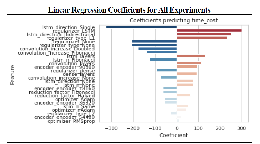
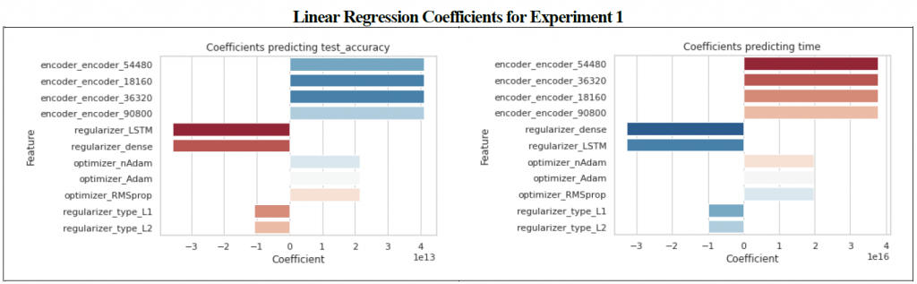
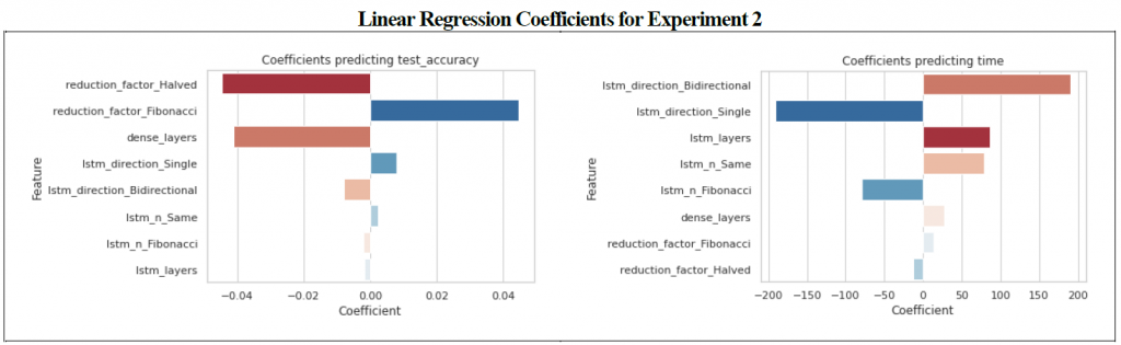
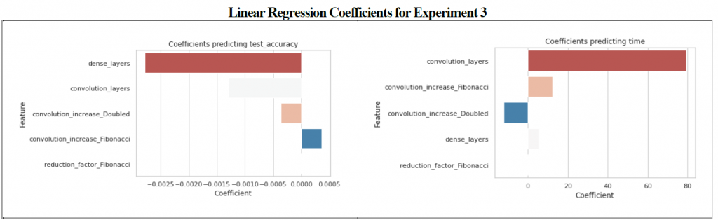
Linear regression models were also created for each experiment using the independent variables in order to predict test accuracy of the data set. Th coefficients from these regression models can help us understand the magnitude of the impact of the variable on accuracy. The charts have been color coded with red indicating that the variable had a negative impact on the desired effect (e.g., a variable which increased time or decreased accuracy) or blue to indicate a positive impact (e.g., a variable which decreased time or increased accuracy). Positive coefficients indicate that the variable increased the value of the predicting variable whereas a negative coefficient decreased the value.
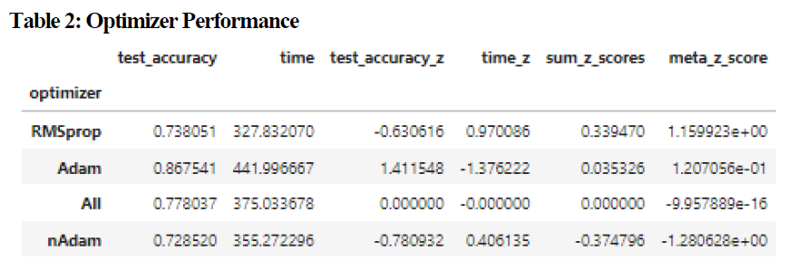
Three optimizers were tested, including RMSprop, Adam, and nAdam. The Adam optimizers had the greatest test accuracy score with an average of 0.867541 (compared with a mean for all optimizers of 0.778037) and a z-score of 1.411548 (Table 2.) This came at the expense of time however, with Adam ranking last (Z-score of -1.37622) and RMSProp having a z-score for training time of 0.970086. The sum of all z-scores resulted in RMSprop having a advantage over Adam (0.339470 to Adam’s 0.035326, with a meta-z score of 1.15 compared with Adam’s meta z-score of 0.12.As a result of this outcome RMSprop was chosen for experiments 2 and 3.
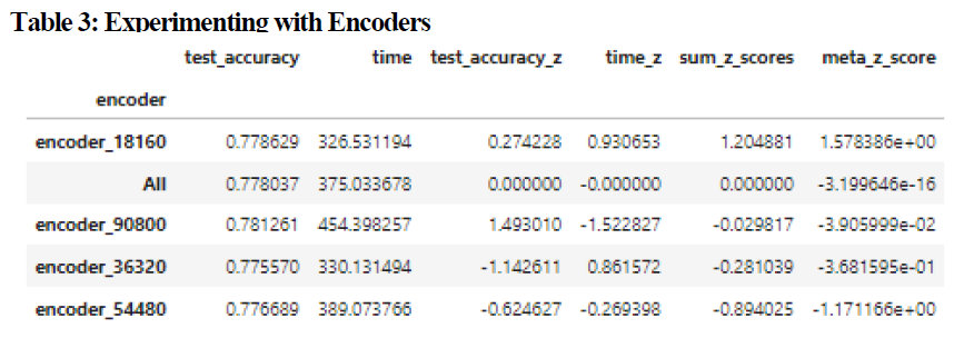
Four encoders were tested in total with a total size of 18160, 36320, 54480, and 90800, using the Fibonacci Scaling. Test accuracy performance between the encoders was negligible with a range of accuracy values between 0.776 and 0.779, and a mean accuracy of 0.778. The encoders however scored significantly different on the convergence time, ranging from 454.398 seconds to 326.531 seconds, with the best performing encoder (encoder_18160) having a z-score of 0.930653, and a total sum of z-scores equal to 1.204881 (the only positive score). The meta z-score was approximately 1.5783, with the next highest score being -1.171166. As a result I did not find a benefit to using a larger encoder for training, and encoder_18160 was used for the remainder of the experiments. Full performance measures can be found in Table 3.
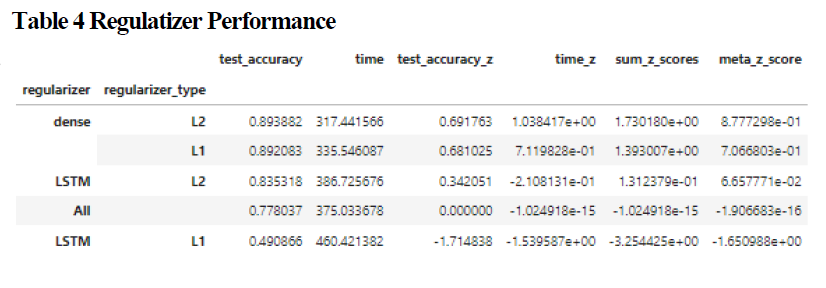
The best regularizer was the L2 regularizer placed on the dense nodes, followed by the L1 regularizer on the dense nodes with accuracy scores averaging approximately 0.89. The worst performing regularizer was the L1 regularizer placed on the LSTM layers. The meta z-score of the dense regularizers were significantly higher than the average (0.8777). Regularization in general had the greatest impact on the reduction of time as seen in Figure 2, however this was in direct proportion to accuracy.
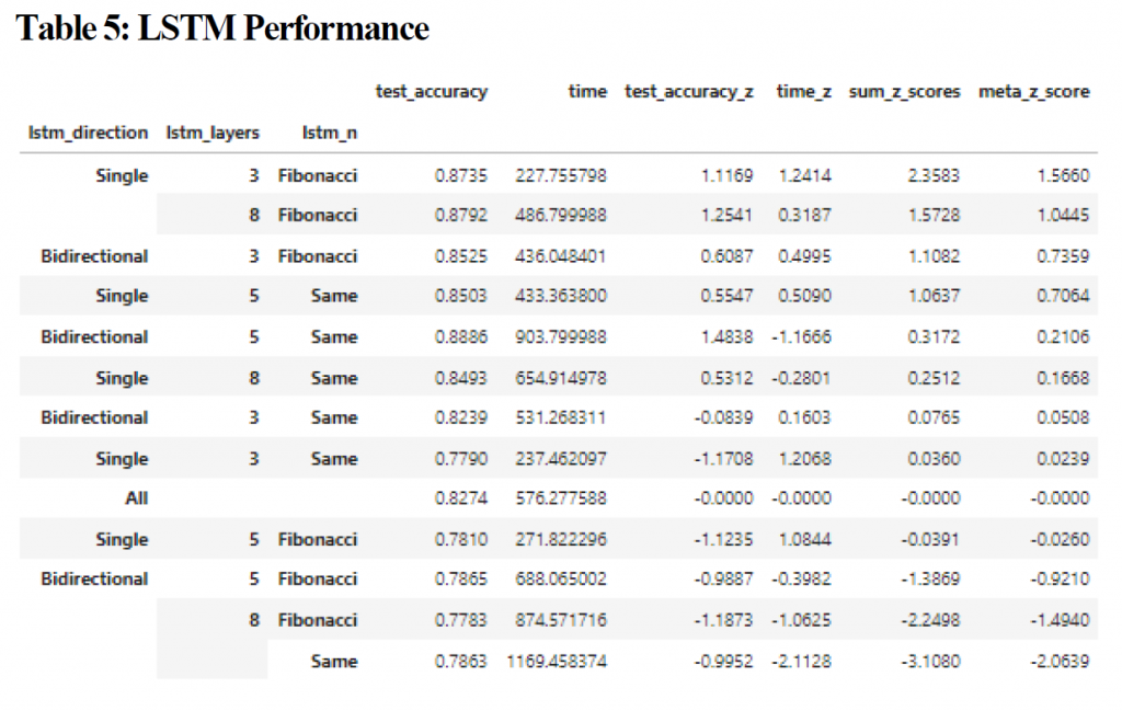
A relatively shallow single LSTM model (3 layers) had the highest Z-score for time (1.1169), whereas a 5 layer Bi-Directional model had the highest z-score for accuracy (1.4838). The best performing model in terms of both time and accuracy was a single directional LSTM model which was comprised of 3 layers utilizing Fibonacci scaling to determine the number of nodes in each successive layer as opposed to all layers having the same number of nodes. An analysis of the effect of node reduction showed that there was virtually no difference between models using the Fibonacci sequence versus models where all layers had an equal number of nodes. There was a real difference in Z-scores however between models which had 3 LSTM layers versus those which had 5 or 8. The sum of the Z-scores for time and accuracy for the 3 layer models was 2.5338 as opposed to -0.1949 and -2.3389 for the 5 and 8 layer models respectfully. The impact on time and accuracy for the LSTM layers relative to experiment 2 can be seen in figure 3.
There was virtually no difference in accuracy for the models based on the number of dense nodes or the kind of reduction method used to calculate the number of nodes per layer with the highest Z-score being 0.5469; there was a difference with the time to converge however with 3 layer models utilizing a halving of the number of nodes for each layer achieving an average time of 514 seconds (z score = 1.0185). The sum of the Z-scores (table 5) however was 1.5654 points, and the meta-z score for the sum of z-scores for the model was only 0.8502, which indicates that while it was statistically significant the significance was minimal.
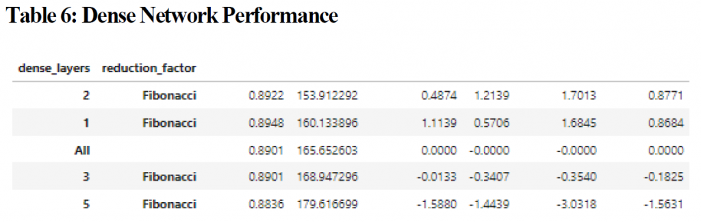
The top performing model contained 2 convolutional layers which increased using a Fibonacci scaling factor and had a z-score of 1.4097 for test accuracy indicating that the difference was statistically different; accuracy performance for this model was 0.8950 on average versus 0.8831 for the worst performing configuration (5 layers with the nodes doubling each layer). Although the z-score was impressive, this represents a variance of only 0.0119 for accuracy. The 2 layer convolutional models which used Fibonacci scaling had a z-score of 0.4711 for time to convergence, which is also low. The combined z-score however was 1.8808, which was statistically significant with a meta-z score of 1.0619. Interestingly, pure deep neural networks (networks with only dense fully connected layers) performed worse than networks with 3 layers in terms of accuracy when combined with convolutional networks, and had the highest negative impact on test accuracy (see figure 3) however when only analyzed by themselves the variance of mean accuracy was less than 0.01 and the best performing class (2 layers) only had a z-score of 0.4874. (see table 6). Unsurprisingly, between dense and convolutional layers, convolutional layers had the greatest impact on the time to convergence (figure 4).
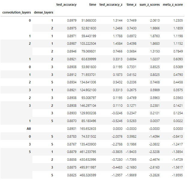
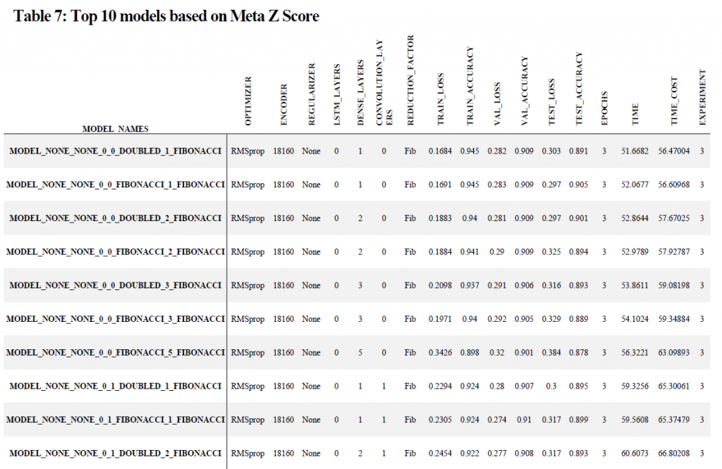
The highest z-score for experiment 1, 2, and 3 respectfully in terms of time cost, or the number of seconds for convergence divided by the mean accuracy (test, validation, and training) for each of the individual models was 0.878978, 0.9331, and 0.7105 respectfully, indicating that there were no models which were significantly different than their respective populations. In terms of the “best” time cost scores across all experiments the simple neural networks had the highest scores (principally due to their very quick training time and generally acceptable accuracy. In other words the complex models where computationally expensive and the time spent to train those models resulted in marginal returns in terms of accuracy. The top 10 models across all experiments are listed in table 7.
Correlations as well as the correlation of correlations were taken for all variables. It is important to note that for this analysis integer variables, such as the number of layers and the number of nodes in each layer, were converted into floats rather than being treated as ordered factors. In looking at the correlations there were no relationships which were not expected. The correlations for each of the three experiments can be seen in the appendix 1.

As we have seen different variables can have very different results on model performance as well as training time. In some cases a more complex or deeper model did not increase model accuracy, and in many cases it increased the training time to such a point as to render the model computationally expensive without a realized gain in accuracy. By creating multiple models and analyzing model performance algorithmically we are able to explore the relationship between many variables that we might not have otherwise been able to do by creating the models manually. A final note on the development of code for the automation of model construction, training, evaluation, and analysis as it relates to the business user. Creating the scaffolding to build models algorithmically takes time, however I encourage the business user to consider the extra time required to create this scaffolding a worthwhile investment as it allows a more thorough understanding of the different impact of model parameters on performance. Algorithmically developed models allow for easy adjustments and simple retraining, and can help to uncover relationships between variables that might not otherwise be found.
Cai, J., Li, J., Li, W., & Wang, J. (2018, 2018-12-01). Deeplearning Model Used in Text Classification. 2018 15th International Computer Conference on Wavelet Active Media Technology and Information Processing (ICCWAMTIP),
Dwivedi, K. D., & Rajeev. (2021). Numerical Solution of Fractional Order Advection Reaction Diffusion Equation with Fibonacci Neural Network. Neural Processing Letters, 53(4), 2687-2699. https://doi.org/10.1007/s11063-021-10513-x
Guo, L., Zhang, D., Wang, L., Wang, H., & Cui, B. (2018). CRAN: A Hybrid CNN-RNN Attention-Based Model for Text Classification. In Conceptual Modeling (pp. 571-585). Springer International Publishing. https://doi.org/10.1007/978-3-030-00847-5_42
Hoijer, H. (1954). The Sapir Whorf hypothesis. In H. Hoijer (Ed.), Language in Culture (pp. 92 – 105). University of Chicago Press.
Li, C., Zhan, G., & Li, Z. (2018, 2018-10-01). News Text Classification Based on Improved Bi-LSTM-CNN. 2018 9th International Conference on Information Technology in Medicine and Education (ITME),
Luwes, N. J. (2010). Fibonacci numbers and the golden rule applied in neural networks. Interim Interdisciplinary Journal, 9(1).
Maqsood, A., Iqbal, U., Shoukat, I. A., Latif, Z., & Kanwal, A. (2021, 2021-01-01). Fibonacci polynomial based multilayer perceptron neural network for classification of medical data. PROCEEDINGS OF SCIEMATHIC 2020,
Merity, S., Keskar, N. S., & Socher, R. (2017). Regularizing and Optimizing LSTM Language Models.
Pinker, S. (1994). The Language Instinct. William Morrow.
Shen, D., Wang, G., Wang, W., Min, M. R., Su, Q., Zhang, Y., Li, C., Henao, R., & Carin, L. (2018). Baseline Needs More Love: On Simple Word-Embedding-Based Models and Associated Pooling Mechanisms.
Shi, M., Wang, K., & Li, C. (2019, 2019-06-01). A C-LSTM with Word Embedding Model for News Text Classification. 2019 IEEE/ACIS 18th International Conference on Computer and Information Science (ICIS),
Turing, A. M. (1950). Computing Machinery and Intelligence. Mind, LIX(236), 433 – 460.
University of Minnesota. (2010). Introduction to Psychology. M Libraries Publishing. https://open.lib.umn.edu/intropsyc
Vedantm, S. (2015). Why We Judge Algorithmic Mistakes More Harshly Than Human Mistakes. Hidden Brain: a conversation about life’s unseen patters. https://www.npr.org/2015/02/03/383454933/why-we-judge-algorithmic-mistakes-more-harsley-than-human-mistakes
Wang, P., Qian, Y., Soong, F. K., He, L., & Zhao, H. (2015). A Unified Tagging Solution: Bidirectional LSTM Recurrent Neural Network with Word Embedding.
![]()
Our purpose is to assist individuals and organizations in making a positive difference in their industry and in their community through education, data strategy, and innovation.
Our mission is to create industry-leading, tailored solutions powered by sound research to assist companies in making data driven decisions and innovating in their field, engaging brilliant people, and cultivating diverse and forward-thinking perspectives.
Chicago, IL
Miami, FL
Kansas City, MO
Salt Lake City, Utah
San Francisco, CA
New York, NY
info@northwesternanalytics.com