Our Research

In part 1 we introduced a manufacturing company that’s seeking to improve their market predictions. Due to the cost of shipping products, the company needs to accurately predict demand two months into the future.

 After trying several data transformations, we found the data may still be non-stationary (have seasonal or other trends). We tried using ARIMA (Autoregressive Integrated Moving Average) which helped reduce autocorrelations, but once again there were likely underlying seasonality components. Finally, we fit our ARIMA model to get a baseline model, returning around a 9% mean absolute percentage error and the predictions didn’t capture the trends in the data well.

In part 2, we apply seasonality models and provide examples using SARIMA (Seasonal Autoregressive Integrated Moving Average), Prophet (an additive model that fits non-linear trends with seasonality and holiday effects), and Holt-Winters (comprised of a forecast equation and three smoothing equations). We will start with SARIMA which uses the same models as ARIMA including auto regressive and moving average with the added benefit of identifying seasonality. 

SARIMA model

To compare the various options, we perform a grid search of SARIMA’s various parameters and check the AIC score to identify the possible best fit for the model. After running the experiments we find SARIMA (0,1,1) (0,1,1,12) has the lowest AIC score. Note: in our ARIMA trials we found ARIMA (0,1,0) performed the best, but in SARIMA we add a moving average order of 1. In our tests we also saw several SARIMA models testing similarly and it’s likely some of the parameters may not be clearly useful. We review the model summary to learn more about what’s going on. 

Figure 1: SARIMA model performance

We then check whether the model generated a good fit to our data and whether it violates any assumptions. In Figure 2, the top left shows the residuals or errors from the model. We don’t see any patterns or trends in the residuals which is what we want to see. The top right histogram reviews the normality of errors and we see the residuals are roughly normally distributed. The bottom left Q-Q plot shows residuals following a linear trend as expected. Lastly, the correlogram shows most of the points in the blue region (the expected range), and although there are one or two fairly high autocorrelations we don’t see any major concerns.

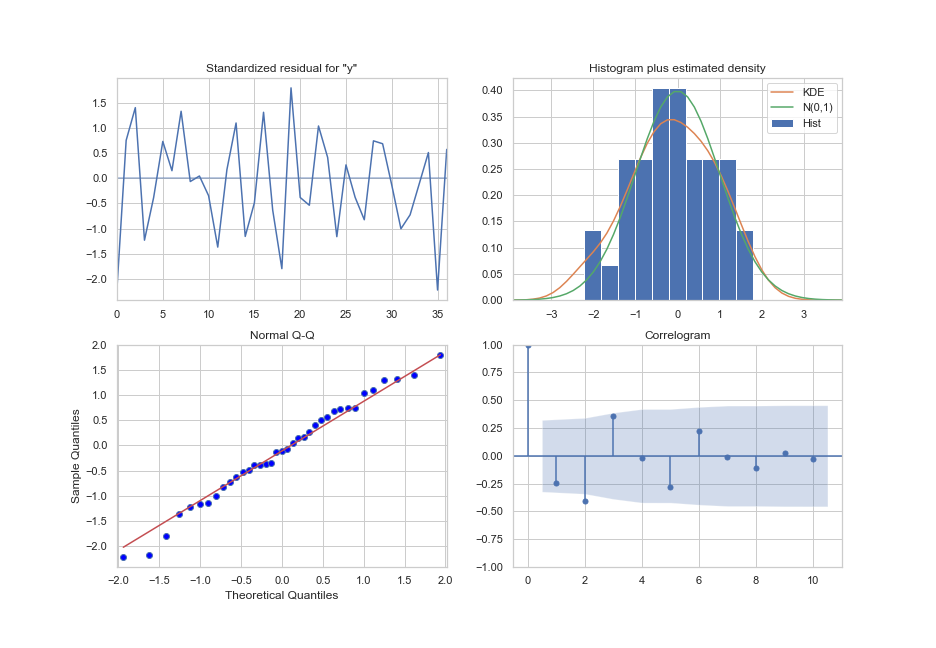
Figure 2: Model diagnostics

Finally, we review how well the model fits the existing data. To do so, we use walk forward validation as we did when testing the ARIMA model in part 1. We make predictions two months into the future, but we add data and refit the model before moving to the third prediction. Using this method we only forecast two months out and for each subsequent month we update the model with new data. The final results of the model are shown in Figure 3 and verify what we expect. With a MAPE of 8.36 the performance has only slightly improved from the ARIMA model and the predictions still diverge quite significantly from the test values.

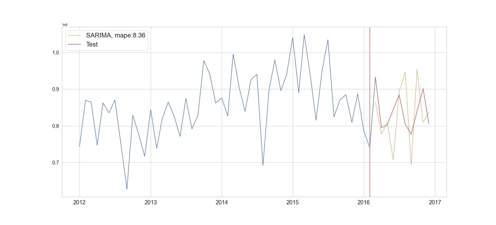
Figure 3: SARIMA forecast

Prophet model

We now turn to Facebook’s Prophet model which can be used on non-stationary, univariate data that supports trend and seasonality. Compared to ARIMA and SARIMA, Prophet is a bit more straightforward to optimize and doesn’t require the iterative process of reviewing the differenced, moving average, and auto-regressor orders. Also, since it can use non-stationary data, there is no need to transform the data as we did previously. Once again we use the walk forward validation method and review the model performance. In Figure 2 we see a much better result than we saw with ARIMA or SARIMA, with a MAPE (Mean Absolute Percentage Error) of 6.09%. While the model struggles with the first few predictions, the predictions are closer to the ground truth – likely due to the model improving as new data is added. 

Figure 4: Prophet forecast

Holt-Winters model

The final model we will try is Holt-Winters, another model for univariate time series data. Holt-Winters uses exponential smoothing in order to give an exponential increasing weight to recent observations. In part 1 we already used simple and double exponential smoothing to attempt to make our data stationary before using the ARIMA model. In the process we showed that simple exponential smoothing didn’t work well for making our data stationary. Double exponential extends beyond simple exponential smoothing by adding a trend component. Finally, there is triple exponential smoothing which adds a third seasonality component. 

The Holt-Winters model has several parameters which require tuning, most of which we could resolve by running the model with different parameters and comparing the performances. However, we also turned to the data and our decomposition graphs to guide in making certain parameter selections. For example, Holt-Winters required providing whether the trend or the seasonality is multiplicative or additive. In short, we need to specify whether the variables are independent. So while the model performed slightly better using a multiplicative seasonality component, the original data suggested there was no clear dependency between the variables and the simpler model was selected. Assuming independence has practical benefits as predictions based on multiplicative properties can quickly get out of hand if the trend changes quickly. The final results for Holt-Winters is shown in Figure 5, performing with a Mean Absolute Percentage Error (MAPE) of 4.8%. 

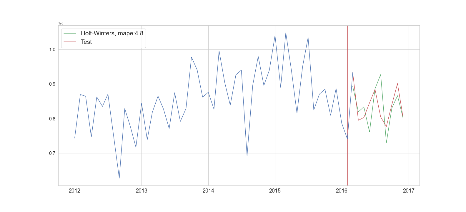
Figure 5: Holt-winters forecast

As a comparison, our original ARIMA model returned a nearly 8% MAPE. Holt-Winters also outperformed Prophet in this particular example. In Figure 6 and 7 we show ten months of predictions for each model to better compare between all of our trained models.

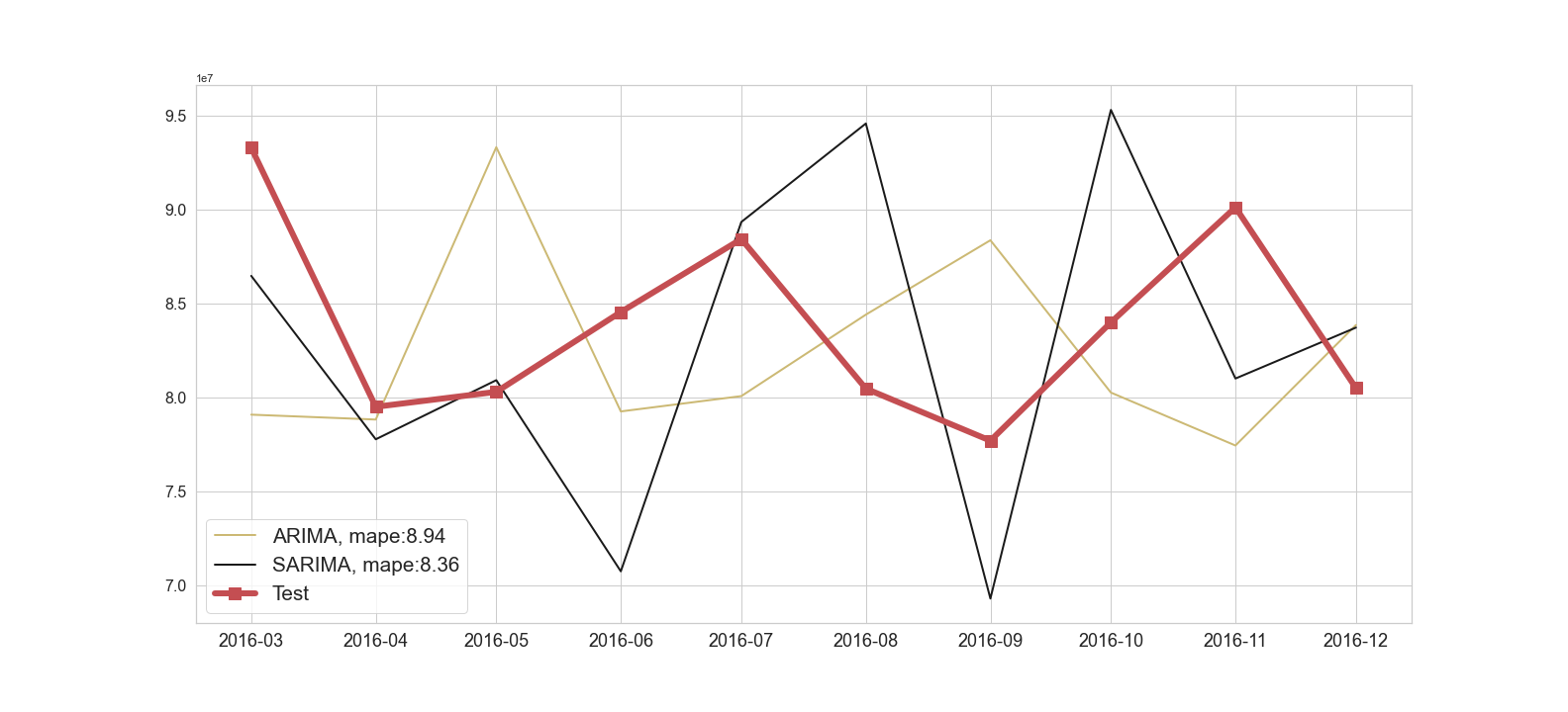
Figure 6: ARIMA and Sarima forecasts

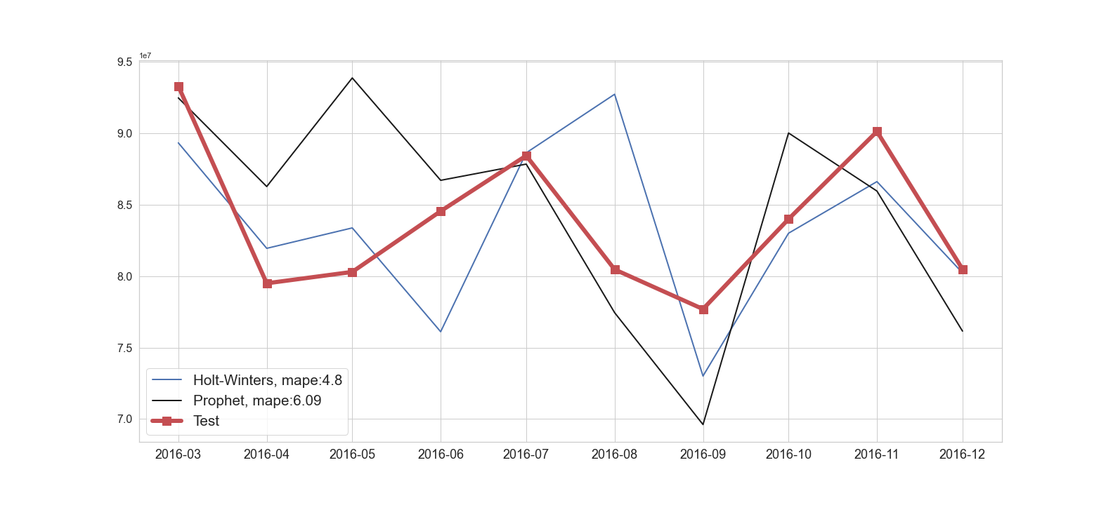
Figure 7: Holt-Winters and Prophet forecasts

Final Words

In this article we demonstrated how we would use seasonal models when there are seasonality components in our univariate data. We demonstrated our process of thoroughly reviewing our model performance, checking any violations in our model assumptions, and detecting issues with the model’s predictions. We also compared multiple seasonal models to capture an optimal fit for our demand forecasting problem. Next we discussed how practical, business, and experimental considerations play a role in selecting a model. Finally, we compared the performances across our different models and reviewed our predictions. Typically, we would have a final step to test our final model on a final hold out set. This final test set is used to provide a more realistic metric of how well our model will perform on new data.

In our example the company needs to start predicting demand on a regular strategy and may need to integrate prediction data in other applications. At this stage we move from the modeling methods we’ve discussed here to implementing and monitoring the models in production. For more information on how we’ve helped companies build and monitor production models, see our case studies or our contact page to schedule a free consultation.