5 Common Challenges with Remote Sensing and How to Tackle Them

November 16, 2020 by

Brennen Chadburn in GIS, Modeling

While remote sensing is not new, recent developments in computer vision have transformed the industry and opened up ample opportunity for industrial and conservation purposes. Computer vision applications are allowing organizations to track deforestation, identify waste, monitor crop health, track urban development, identify valuable resources, and solve a myriad of similar problems. Remote sensing doesn’t come without its set of challenges. We identify a few of the most challenging remote sensing obstacles in image classification and demonstrate how we can help companies address them including:

Atmospheric correction
Dealing with multi-spectral images
Locating satellite images
Labeling images
Building models for classifying multi-spectral images

1. Atmospheric correction

Computer vision applications typically include classifying objects and in remote sensing it’s no different. We may need to track changes over time, compute density and object size (image segmentation), identify anomalies, but the heart of our problem is object classification. Computer vision problems typically start with image processing including steps such as data augmentation, image resizing, and normalization. Similarly, satellite images typically require a special type of image processing called atmospheric correction.

Satellite imaging picks up on radiation reflected back from clouds and the earth’s surface (i.e. top-of-atmosphere or TOA reflectance) and the spectral reflectance can be drastically impacted by differences in the atmosphere. Atmospheric correction tries to remove the light reflected from the atmosphere and leave us with the surface reflectance.

Know your problem

As is often the case, the solution depends on your specific application. If conducting exploratory work only, or if images come from the same location and time, atmospheric correction may not even be helpful. While images from different locations around the globe may require more intensive corrections. It often helps to try a few methods and compare the differences. Below are a few questions to consider:

- Are you using images from different times? Atmospheric correction is needed.
- Are images from locations in different parts of the globe? Atmospheric correction is needed.
- Are you detecting objects on land or ocean? Images from the ocean can be severely impacted by moisture in the air. Some atmospheric corrections such as QUAC need lots of variety in the scene to apply correction properly and may not work well for oceans. In a recent research article¹, l2gen and Sen2cor performed worse in the ocean than C2RCC, iCOR, Polymer and Acolite.
- Do objects include vegetation? If so, it depends on the spectral indices (we will review these more later) needed for classification and if they are sensitive to atmospheric correction.
- Accuracy required by the model and difficulty of the problem. Sometimes only light atmospheric corrections are required to provide the results needed. Lighter weight corrections allow faster processing time which can be critical when processing multiple spectrums or lots of images. Some light-weight corrections include Acolite and DOS1. Otherwise, you might try corrections such as Sen2cor, Flaash, or Maja.
- What type of sensors are we using? We may be dealing with Multi-spectral images, hyperspectral, super-spectral etc. For multi-spectral: consider Quacas a light-weight solution which can work just as well for multi-spectral images compared to even heavy duty corrections. Hyperspectral or super-spectral include visible and non-visible spectrums impacted by reflectance. Some correction is needed and depending on the application more intensive correction could be warranted.

2. Locating Satellite images

If this isn’t one of your challenges, feel free to skip to the next section. However, for many organizations, locating enough satellite images to train computer vision models or making classifications can be particularly challenging. To determine where to look for relevant images, below are a couple questions you should consider.

How frequently do we need to be classifying objects in a given location?

If we don’t have to come back to the same location daily, we can try using publicly available satellite images such as landast or sentinel which you can find at Open Access Hub, Onda Catalogue or one of the other available open-source platforms. Some landsats have 16 day repeat cycles while sentinel 1&2 have 5 and 6 day repeat cycles respectively. If you need images more frequently, you can consider paying commercial satellite companies for images. For most applications, it makes sense that whatever platform you decide on, you stick to that platform for image classification as the models will need to be trained on images of the same size, resolution, and spectrums.

What resolution is required for our application?

For many applications, 10 or even 20 meter pixel resolution is sufficient and is typically available with open source satellite images. Higher resolutions, most commonly 3 or 5 meter resolution images, can be acquired from commercial satellite companies. Given the expense of working with commercial satellite companies we recommend first evaluating what can be detected with open source images. First, classification models may need much lower resolution than expected; depending on the context, certain spectral bands as well as contextual clues can help inform the models’ classification. Furthermore, models can be used to identify areas of concern to greatly reduce what areas need higher resolution or need investigation. In fact, some companies conduct anomaly detection at higher resolution and take action on the ground as needed to investigate further.

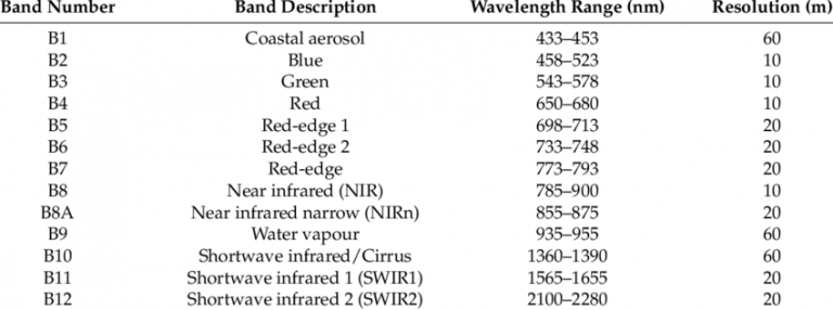
Table 1: Spectral bands and resolutions of Sentinel-2 MSI sensor.3

3. Dealing with multispectral images

Similar to how a color image includes red, green, and blue values – multispectral images report on image values for various wavelengths across the electromagnetic spectrum. Some satellites report on only a few of these spectral bands while satellites such as Sentinel 2 report on 13 different wavelengths. It’s unlikely for a single application to need to use each wavelength. Instead, we recommend determining which wavelengths are well-suited for the objects you need to classify. For mineral deposits you may need to focus on thermal infrared, but if seeking to separate soil and vegetation, blue may be needed. Once you have limited the number of potential color bands, you can even create what are called false color images. False color images are color composites that don’t reflect the normal combination of red, green, and blue. Instead, we can combine near infrared, green, and red to better detect vegetation health or shortwave infrared, near infrared, and green to identify recently burned ground2.

Finally, review the current scientific literature for useful spectral indices for your application. Spectral indices are designed to discriminate between particular objects. For instance, NDVI (normalized difference vegetation index) is particularly useful for live green vegetation. Rather than looking at multiple bands as we talked about with false color images, NDVI (and other spectral indices) returns a single value for each pixel with high NDVI values corresponding to vegetation. We can even develop our own indices for unique objects once we identify applicable spectrums.

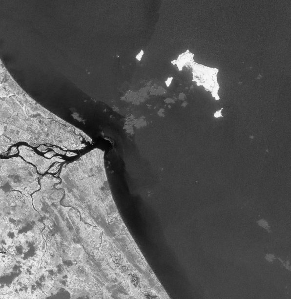
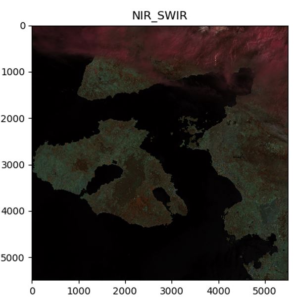
Fig 1: NDVI image. Brighter pixels indicate high values associated with vegetation

Fig 2: False color image. The image replaces the usual RGB color bands with near infrared and short-wave infrared color bands to highlight different features of the image.

4. Labeling

Computer vision models require object labels to train and learn to classify objects. Getting accurate labels is particularly difficult with satellite imaging for several reasons. Below are two common difficulties in labeling we will address.

Verifying objects not easily distinguishable
Finding ‘rare’ or infrequent objects in large images

Verifying objects

Having boots on the ground to verify objects can be impractical and expensive. Alternatively, there are several options to help reduce costs and label images properly. There are many platforms out there for labelling images such as Labelbox, LabelMG, and Supervise.ly. However, they can come with platform license fees, consulting fees, and hourly labeling rates. If you don’t require as much hand holding though, we have found that mechanical turk services can be easy to use, integrate well with AWS platform, and are much less expensive than aforementioned platforms. You can submit labeling jobs with a set of examples and have multiple people labeling the same images to ensure high accuracy.

Conduct the labeling in-house. When working on a budget, or working with objects requiring looking at multiple spectral bands (not just true color aka RGB images) it may make sense to bring labelling in house. Sometimes you can only label an object by viewing the object in different spectral wavelengths, false color images, or specific spectral indices. In this case, it can end up being simpler than handing it off and trying to explain the labelling process. Furthermore, before building models, it’s going to be critical to understand which spectrums and spectral indices are likely to be helpful so it may be an essential step to know what features to use in the model.

Finding rare or infrequent objects

When conducting labeling, we may only be interested in areas that have changed recently. If so, we can locate areas where the spectral signatures have changed significantly. We can also use spectral signatures to identify types of objects. Some objects have extremely high or low values for certain indices or for specific wavelengths. Process the image and find pixels that lie within the spectral range expected for an object. What’s left is a much smaller amount of images to review manually. As mentioned in the section on labeling, objects have specific spectrums that are useful as well as indices which helps separate them. For instance, as discussed earlier, NDVI is often used for vegetation classification. When NDVI values are low, pixels are less likely to represent vegetation and, in some applications, we can ignore significant areas of the images with low NDVI values. In essence, we use spectral signatures to identify coordinates we are interested in for a given image. We then export images for labeling – such as a 128×128 pixel image – centered around those identified coordinates. As a word of warning, filtering out images can bias your classification model if your filtering is overly aggressive or misrepresents the distribution of image types that will need to be classified.

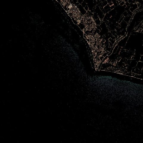
Fig 3: Shows an image where we’ve filtered out pixels that haven’t changed significantly from previous images. Next, we can filter out pixels based on the objects of interest. For instance, if looking for vegetation, its likely almost all of the pixels in the ocean (area without brown pixels) would be left out. Note, filtering in this manner is for demonstration purposes only. In reality, we are filtering for specific coordinates so we know what portions of the image to extract for labeling.

5. Building models for classifying multi-spectral images

At this point in the process, we have identified useful false color images as well as indices that may be helpful for classification. We have now completed labeling which will apply to any set of false color images we create for a given image. The next challenge is how we build an image classifier to apply to multi-spectral images.

In the case where we have a true color image (TCI) or a false color image consisting of three colors you can build on pre-trained models to conduct image classification such as Nasnet, ResNet or Inception. We train the model with these images just as we would with other RGB images. There is a lot of material on this portion of modeling so I won’t review these steps in detail here.

In the case where multiple color images are needed for classification, more advanced methods would be required. You could use ensemble methods (multiple models), and stacked models (multiple models are inputs into another model) to incorporate several images in order to make a final prediction. If you are wanting to incorporate spectral indices, pre-trained models can be built upon to allow multiple inputs. In this case, indices would be added in one of the latest layers of the model rather than being added as additional channels/colors; allowing the model to still create high level image features from the color image, while also taking into consideration the spectral index values before classifying the image.

Before taking on these steps, ensure the model is learning before adding other features or several layers to the pre-trained model. Small iterative changes are key once you’ve established a working base model. Only then can we know if architectural changes are helping or if a particular index doesn’t improve the model’s accuracy. Of course, once we get to that point, try other related indices or better yet try a combination (with each index added as separate inputs into the model) to see if it improves the model accuracy. Be sure to try a variety of spectral bands and indices to find an optimal solution. Refining models can be particularly challenging especially with multi-spectral images given the variety of options. However, if you make iterative changes, measure performance changes, and explore outputs to understand the model improvements, you can avoid a lot of headache and quickly make large improvements to the model’s performance.

Final words

In this article, we’ve reviewed several common challenges in remote sensing. It is far from an exhaustive list and while so much more could be said about each of these challenges, hopefully it can provide some guidance and assistance in your journey in remote sensing. Feel free to leave a comment or ask any questions you may have. For more information about Northwestern Analytic’s work in remote sensing or to learn more about how we can help your company don’t hesitate to reach out.

Reference

1 https://www.sciencedirect.com/science/article/pii/S0034425719301099

2 https://earthobservatory.nasa.gov/features/FalseColor/page6.php

3 Hawrylo, Pawel & Wezyk, Piotr. (2018). Predicting Growing Stock Volume of Scots Pine Stands Using Sentinel-2 Satellite Imagery and Airborne Image-Derived Point Clouds. Forests. 9. 274. 10.3390/f9050274.

About the Author

Contact Us

Our Research

5 Common Challenges with Remote Sensing and How to Tackle Them